Station P612

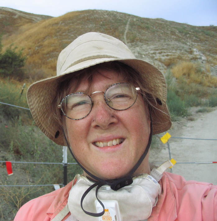
Questions for Sally McGill

How did you become a scientist/engineer?

As a high school student, when I started thinking about possible careers I realized that I liked being outside and I liked working with maps. My family had done a lot of canoe camping in northern Minnesota, and I had enjoyed being the navigator, matching up the bays and peninsulas on the map with those that I could see in front of me from the vantage point of our canoe. I loved the sense of discovery and exploration of the natural world. These interests led me into geology, where I have continued to explore mountains and deserts, learning how to listen to the stories told by the landscapes and rock formations around me.

What is your job like?

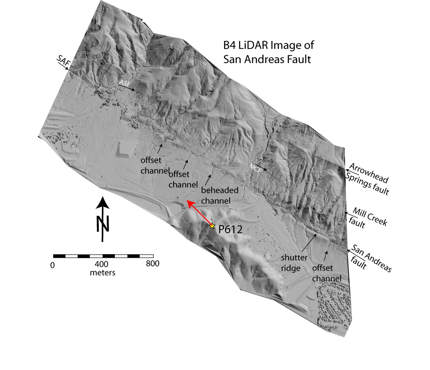
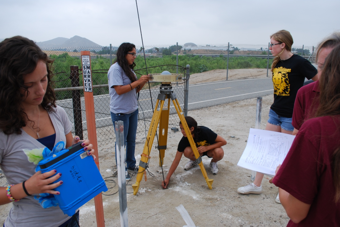
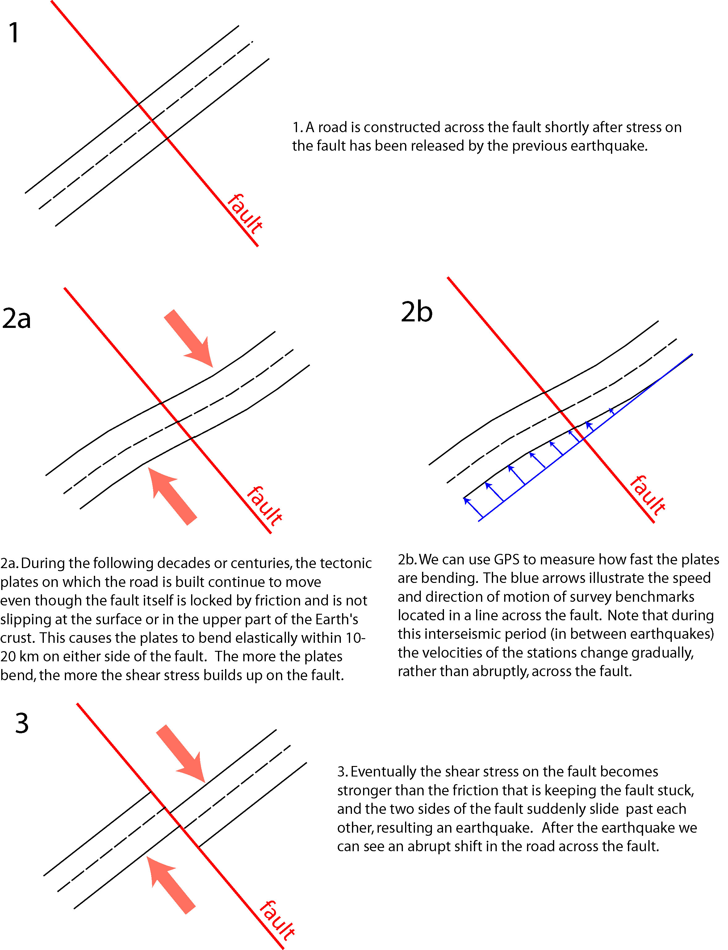
I am a geology professor at California State University, San Bernardino. When I was in college I had told myself that I didn't want to have the same career my whole life. But I have found such variety in the work I do as a university professor that I have not yet run out of new things to do. I teach a variety of courses on geology, and I conduct research on the San Andreas Fault and other active faults. I often begin my research projects by looking at aerial photographs and other remote sensing images, like LiDAR. I look for landforms that have been laterally offset by the fault, such as stream channels or alluvial fans. My students and I then spend time out in the field, making geologic maps of those offset landforms and looking for ways to measure their age so that we can determine how long it took for those features to become offset.

What are you hoping to learn from your research?

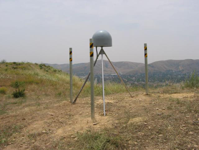
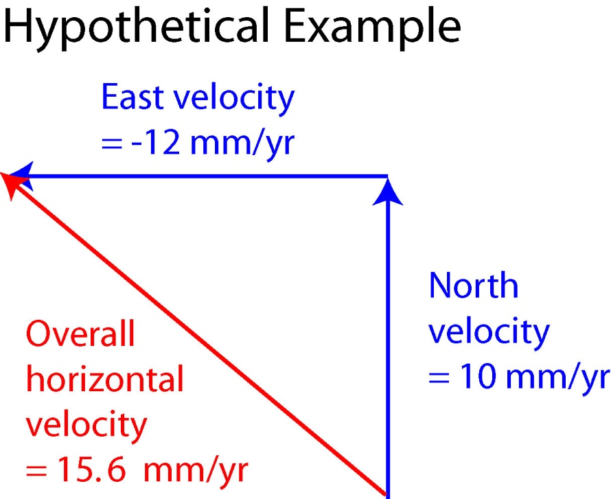
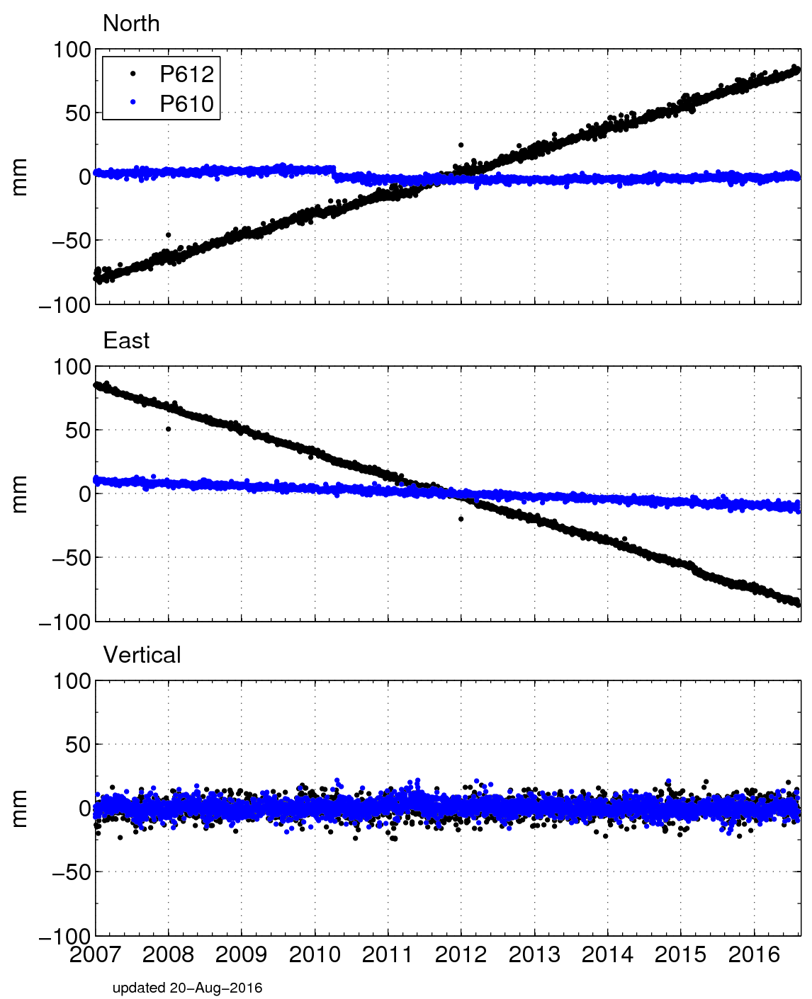
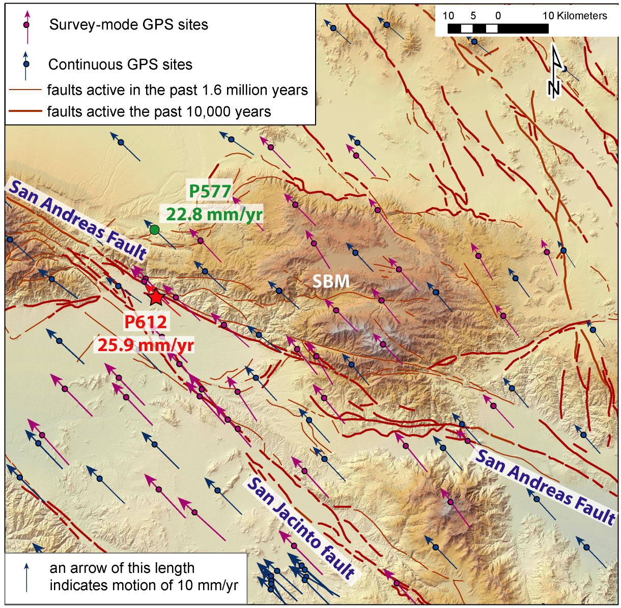
A primary goal of my research is to measure how fast the San Andreas Fault and other faults are moving. Using offset landforms, as described above, we can measure the long-term fault slip rate, averaged over thousands of years, as a result of many earthquakes. GPS gives us another, independent method of estimating fault slip rates. With GPS we can measure the bending of the tectonic plates over the past 10-20 years and then infer what rate of slip on the deep part of the fault, where the rocks are hot enough to flow, would cause the degree of bending that we observe at the surface using GPS. Knowing how fast the faults are moving is a vital piece of information for estimating the earthquake hazards of a region.

San Andreas Fault

P612 is about 460 meters southwest of the San Andreas Fault. A number of stream drainages are offset right-laterally by the San Andreas Fault in this area, as can be seen in Figure 1. Both the offset drainages and the GPS time series (Figure 2) show that P612 is moving north and west relative to the North American plate. Figure 3 shows the motion of P612 in the context of other continuously monitored GPS sites in southern California. The lengths of the arrows represent the speed of each site relative to the stable interior of the North American plate. In Figure 3, you can see that there is NOT an abrupt change in the speed of the sites as you cross the San Andreas Fault. Instead, the speed of the sites increases gradually as you cross the network of faults that makes up the boundary between the North American and Pacific plates. In part this is due to the broad width of this complex network of faults. But even if the San Andreas Fault were the only fault in the plate boundary, the arrows would still only change their length gradually in the vicinity of the fault rather than changing their length abruptly across the fault. The reason for this is that the San Andreas Fault has been locked during the entire time that these GPS stations have been operating (for the past 10-20 years). This means that, at the surface (and within the top 15 km or so of the Earth's crust), there has been no slippage along the San Andreas Fault since the last major earthquakes, more than 150 years ago.

At a broader scale, the Pacific plate has still been moving northwestward relative to the North American plate during this time, and this has caused both the Pacific and North American plates to bend in the vicinity of the San Andreas Fault (and of other faults within the plate boundary zone) (Figure 4). In addition, gradual creep along the deep part of the San Andreas Fault (below about 15 km depth) has probably been occurring as the hot rocks at those depths flow past each other along the fault. This also contributes to the bending at the surface of the Earth that we can observe by noting the gradual change in the lengths of the arrows across the plate boundary in Figure 3. GPS data from continuously operating sites can be supplemented with GPS data collected from portable GPS equipment that is set up temporarily and moved from site to site. These additional data give us a more detailed picture of how the surface of the Earth is deforming near the faults. CalState University San Bernardino geology majors and local high school science teachers and their students have helped to collect such GPS data in the vicinity of the San Bernardino Mountains over the past 10 years (Figure 5), contributing to our understanding of the San Andreas Fault in this region (Figure 6).

In addition to telling us about tectonic deformation around the San Andreas Fault, P612 is also being used to study vegetation growth; see this site for the vegetation-related records for P612.

Spotlight Questions